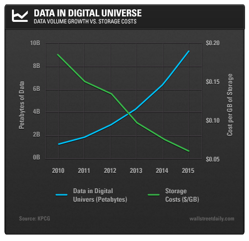
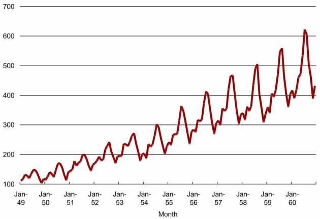
 When we have a series of data points indexed in time order we can define that as a “Time Series”. Most commonly, a time series is a sequence taken at successive equally spaced points in time. Monthly rainfall data, temperature data of a certain place are some examples for time series.
In the field of predictive analytics, there are many incidents that need to analyze time series data and forecast the future values of that based on the previous values. Think of a scenario where you’ve to do a time series prediction for your business data or an incident where part of your predictive experiment contains a time series field that need to predict the future data points… There are many algorithms and machine learning models that you can use for forecasting time series values.
Multi-layer perception, Bayesian neural networks, radial basis functions, generalized regression neural networks (also called kernel regression), K-nearest neighbor regression, CART regression trees, support vector regression, and Gaussian processes are some machine learning algorithms that can be used for time series forecasting.
See here for more about these methods
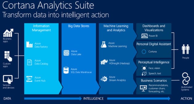
Autoregressive Moving Average (ARIMA), Seasonal-ARIMA, Exponential smoothing (ETS) are some algorithms that widely used for this kind of time series analysis. I’m not going to dig deep into the algorithms, trend analysis and all numbers & characteristics bound with time series. Just going to demonstrate a simple way that you can do time series analysis in your deployments using Azure ML Studio.
After adding a dataset that contains a time series data into AzureML Studio, you can perform the time series analysis and predictions by using python or R scripts. In addition to that ML Studio offers a pre-built module for Anomaly detection of time series datasets. It can learn the normal characteristics of the provided time series and detect deviations from the normal pattern.
Here I’ve used forecast R package to write code snippets enabling AzureML Studio to do TS forecasting using popular time series algorithms namely as ARIMA, Seasonal ARIMA and ETS.
ARIMA seasonal & ARIMA non-seasonal
#ARIMA Seasonal / ARIMA non-seasonal
library(forecast)
# Map 1-based optional input ports to variables
dataset1 <- maml.mapInputPort(1) # class: data.frame
dataset2 <- maml.mapInputPort(2) # class: data.frame

#Enter the seasonality of the timeseries here
#For non-seasonal model use '1' as the seasonality
seasonality<-12
labels <- as.numeric(dataset1$data)
timeseries <- ts(labels,frequency=seasonality)
model <- auto.arima(timeseries)
numPeriodsToForecast <- ceiling(max(dataset2$date)) - ceiling(max(dataset1$date))
numPeriodsToForecast <- max(numPeriodsToForecast, 0)
forecastedData <- forecast(model, h=numPeriodsToForecast)
forecastedData <- as.numeric(forecastedData$mean)

output <- data.frame(date=dataset2$date,forecast=forecastedData)
data.set <- output

# Select data.frame to be sent to the output Dataset port
maml.mapOutputPort("data.set");
ETS seasonal & ETS non-seasonal
#ETS seasonal / ETS non-seasonal
library(forecast)
# Map 1-based optional input ports to variables
dataset1 <- maml.mapInputPort(1) # class: data.frame
dataset2 <- maml.mapInputPort(2) # class: data.frame

#Add the seasonality here
#Assign seasonality as 'a' for non-seasonal ETS
seasonality<-12
labels <- as.numeric(dataset1$data)
timeseries <- ts(labels,frequency=seasonality)
model <- ets(timeseries)
numPeriodsToForecast <- ceiling(max(dataset2$date)) - ceiling(max(dataset1$date))
numPeriodsToForecast <- max(numPeriodsToForecast, 0)
forecastedData <- forecast(model, h=numPeriodsToForecast)
forecastedData <- as.numeric(forecastedData$mean)

output <- data.frame(date=dataset2$date,forecast=forecastedData)
data.set <- output

# Select data.frame to be sent to the output Dataset port
maml.mapOutputPort("data.set");
The advantage of using R script for the prediction is the ability of customizing the script as you want. But if you want looking for an instant solution for doing time series prediction, there’s a custom module in Cortana Intelligence gallery to do time series forecasting.
https://gallery.cortanaintelligence.com/Experiment/Time-Series-Forecasting-using-Custom-Modules-1
You just have to open that in your studio and re-use the built modules in your experiment. See what’s happening to your sales in next December! 🙂
 Data science is one of the most trending buzz words in the industry today. Obviously you’ve to have hell a lot of experience with data analytics, understanding on different data science related problems and their solutions to become a good data scientist.


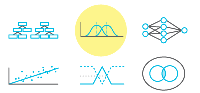
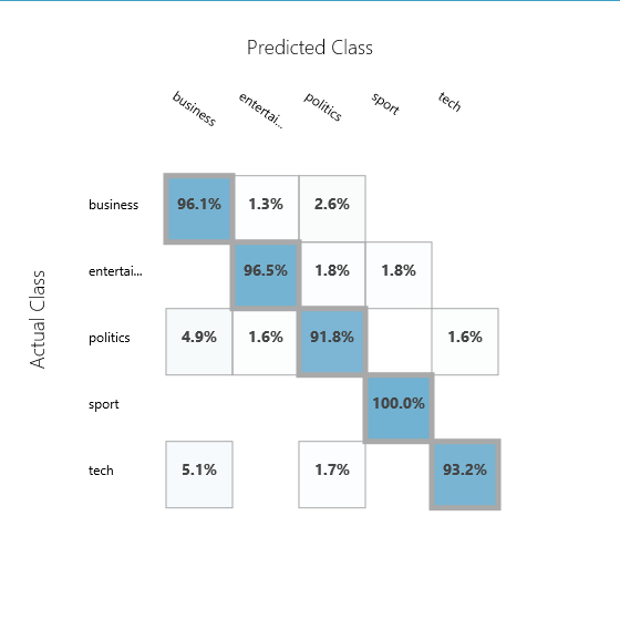
 Classification is one of the most popular machine learning applications used. To classify spam mails, classify pictures, classify news articles into categories are some well known examples where machine learning classification algorithms are used.


 With the power of cloud, we going to play with data now! 🙂
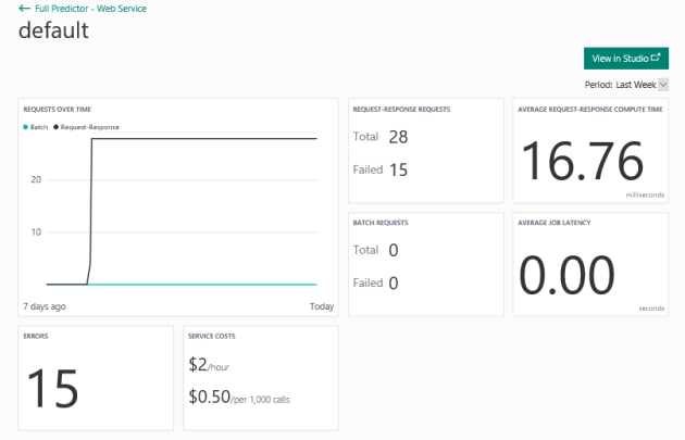
 You can use AzureML absolutely for free. But if you want to deploy a web service and play with serious tasks have to go for an appropriate subscription. If you have a MSDN subscription, you can use it here 🙂
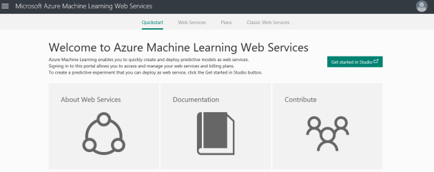
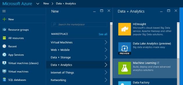 In the portal go for new -> data + analytics -> Machine Learning
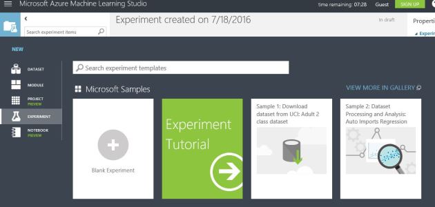 Now you are there! Click on the new -> Blank experiment!